EXCEL - Help appreciated!

[GE90]

As most users I guess, I just use trial and error (following Google searches) when working with Excel!

However, I have a specific requirement that I cannot work out, and would appreciate any input!

So, I have a shares spreadsheet - sounds fancy, but not much value, just some fun really.

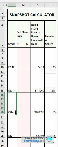
I have the share names in a column, and I have another column in which I have the break even share price, based on my purchase price and costs etc. All good.

However, as I purchased a number of batches of say EasyJet shares over a couple of years, I would like to take an average of this break even column. I researched how, BUT......

As I have a few different shares, I would like a formula like this:

If the selected cells have EZJ in the text, then add this one to the average formula. Help with the whole formula (less cell numbers!) would be very welcome.

Thanks

[Meeten-5dulx]

=if(cell ="EZY",Average!A1:A2),"")

Assuming the average price of the EZY shares are in A1, A2
or hcange to have the average price in a particular cell, and rename as EZY_Ave_Price

Does that help?

[GE90]

Thanks very much.

So where does the range of cells go to search for the text?

Cheers

[Jaguar99]

Have a look at the AVERAGEIF function

The tooltip will tell you exactly what you need to fill in as you type

[GE90]

Sorry to sound dim, but this is what I have tried, but I receive an error:

=if(L6:L60="EZY",Average!N6:N60),"")

Where L6:L60 are the cells with the text, and N6:N60 are the cells with the break even share price.

I had trouble working out the function help tool......

Thanks

[Dingu]

GE90 said:

Sorry to sound dim, but this is what I have tried, but I receive an error:

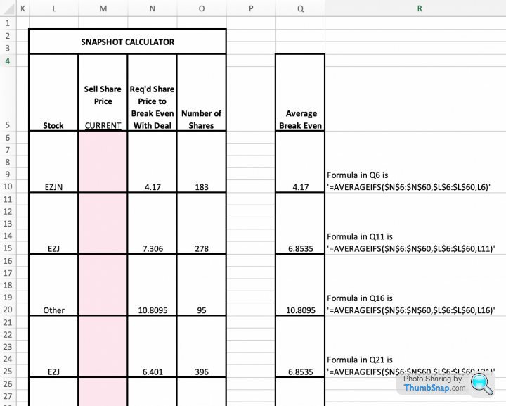
=if(L6:L60="EZY",Average!N6:N60),"")

Where L6:L60 are the cells with the text, and N6:N60 are the cells with the break even share price.

I had trouble working out the function help tool......

Thanks

=AVERAGEIFS(N6:N60,L6:L60,”EZY”)

[Jaguar99]

GE90 said:

Sorry to sound dim, but this is what I have tried, but I receive an error:

=if(L6:L60="EZY",Average!N6:N60),"")

Where L6:L60 are the cells with the text, and N6:N60 are the cells with the break even share price.

I had trouble working out the function help tool......

Thanks

=AVERAGEIF(L6:L60,”EZY”,N6:N60)

[GE90]

Thanks - now get the following error!

How to correct a #DIV/0! error

[Dingu]

GE90 said:

Thanks - now get the following error!

How to correct a #DIV/0! error

That should only be happening if it is dividing by 0, so in the averageif (or averageifs) it would occur if no instances of the condition (EZY) have been found.

Are there any spaces before or after the EZY in the cells in L6 to L60?

[GE90]

[GE90]

Ah, typo! Sorry, let me try again!

[GE90]

Still the same error after correcting the share code.

I've also changed the share code cells to text, as this was not the case!

Any thoughts - again, thanks!

[GE90]

The break even share price is set as currency - hope this is OK?

Thanks

[mmm-five]

Post the actual formula you've put in...but is there a reason for all the blank rows between entries?

BYW, would a simple average of break-even prices even work if you've got different amounts of shares in multiple tranches?

e.g. you have 100 shares that need £6 break even (so £600), and 1000 that need a £4 break even (so £4000). This would nominally give you an average £5 break even for all 11000 (so £5500)...whereas it should be (100@£6 + 1000@£4) / 1100 = £4600...so a £4.18 average not £5.

Edited by mmm-five on Saturday 14th January 16:45

[GE90]

=AVERAGEIFS(N6:N60,L6:L60,”EZJ”)

Sorry, not sure what is meant by the rows observation. I have merged cells if that helps?

Thanks

[GE90]

The reason they are merged here is because a column further along needs the individual rows

[GE90]

mmm-five said:

Post the actual formula you've put in...but is there a reason for all the blank rows between entries?

BYW, would a simple average of break-even prices even work if you've got different amounts of shares in multiple tranches?

e.g. you have 100 shares that need £6 break even (so £600), and 1000 that need a £4 break even (so £4000). This would nominally give you an average £5 break even for all 11000 (so £5500)...whereas it should be (100@£6 + 1000@£4) / 1100 = £4600...so a £4.18 average not £5.

Edited by mmm-five on Saturday 14th January 16:45

My head hurts!

[mmm-five]

GE90 said:

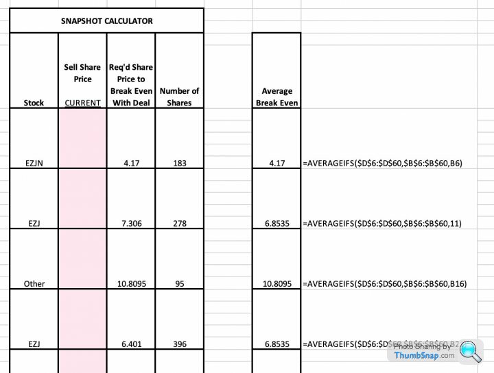
=AVERAGEIFS(N6:N60,L6:L60,”EZJ”)

Sorry, not sure what is meant by the rows observation. I have merged cells if that helps?

Thanks

All I can think of is that one of the value in one of those merged cells are not in the same row as the price (even if it looks like it is)...so the average sees the "EZJ" in one row of column L, and no corresponding breakeven price in the same row of column N.

Normally, when a cell is merged, the value is stored in the top-left cell, but in the 'EZJ' one in L15, when you click on the item does it reference L15 or L11? I'm just wondering if something is formatted to look like it's merged, when it's not?

Edited by mmm-five on Saturday 14th January 16:54

[mmm-five]

GE90 said:

My head hurts!

Try this...

=AVERAGEIFS($N$6:$N$60,$L$6:$L$60,L6)

You can copy & paste the formula from the first entry down into the others, and it will change the 'L6' in the formula as per the cells shown in the last column.

Edited by mmm-five on Saturday 14th January 17:29

[GE90]

mmm-five said:

Try this...

=AVERAGEIFS($D$6:$D$60,$B$6:$B$60,B6)

You can copy & paste the formula from the first entry down into the others, and it will change the 'B6' in the formula as per the cells shown in the last column.

Edited by mmm-five on Saturday 14th January 17:11

Really sorry, I'm lost!