Excel : highlight cells containing number

[r3g]

Hi, google is giving me results for everything except what I want. My column A has cell data where a handful of cells are alphanumeric, eg. AA3, BY4, C6T, 8MJ. The vast majority are just 3 letters. I don't need to filter them out into a separate sheet or anything, I just want a way of highlighting them so I can scan down the sheet and note them. Is there a way of doing this in Excel? Google is only giving me results if the cell only contains numbers, which is no use to me. Thanks.

[fbc]

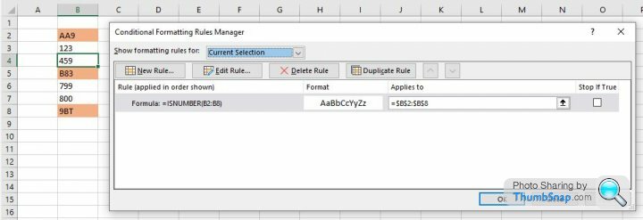
You could use the ISNUMBER function as a Conditional Formatting rule to highlight cells that are numeric, meaning your non-highlighted cells will be those containing at least one letter. Or, if you want those non-numeric cells to stand out, format the entire column with a coloured fill (e.g. orange), and set the conditional formatting rule to apply no cell fill to those cells which are purely numeric, that way your cells with at least one letter will remain orange and those cells that are purely numeric will have no fill.

Edited by fbc on Wednesday 23 November 08:39

[r3g]

fbc said:

You could use the ISNUMBER function as a Conditional Formatting rule to highlight cells that are numeric, meaning your non-highlighted cells will be those containing at least one letter. Or, if you want those non-numeric cells to stand out, format the entire column with a coloured fill (e.g. orange), and set the conditional formatting rule to apply no cell fill to those cells which are purely numeric, that way your cells with at least one letter will remain orange and those cells that are purely numeric will have no fill.

|https://thumbsnap.com/KWPfQMNC[/url]

Edited by fbc on Wednesday 23 November 08:37

Thanks, but that's the exact problem I have with my google searching. All the cells contain letters, basically AAA through ZZZ, but there's maybe a couple of dozen or so which are alphanumeric. No cells are just numbers, so the "ISNUMBER" conditional formatting unfortunately doesn't work either way around.

[fbc]

Ah, apologies for misreading.

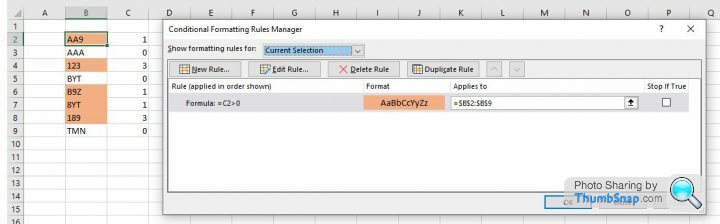
This isn't as neat (I'm sure there must be a more elegant way to do this), next to your column of data, put this formula in:

=COUNT(FIND({0,1,2,3,4,5,6,7,8,9},B2))

That will produce a value of 0 where only letters are in the cells, and a value of 1 or higher where at least one number exists. Then reference that cell in the Conditional Formatting rule:

[r3g]

fbc said:

Ah, apologies for misreading.

This isn't as neat (I'm sure there must be a more elegant way to do this), next to your column of data, put this formula in:

=COUNT(FIND({0,1,2,3,4,5,6,7,8,9},B2))

That will produce a value of 0 where only letters are in the cells, and a value of 1 or higher where at least one number exists. Then reference that cell in the Conditional Formatting rule:

I might be doing something wrong. I have created a new column B and all the other columns (which mostly contain numbers) are shifted across by 1 column. When posting the formula in B2 it gives a Circular Reference Warning. Then puts 0 in the cell and nothing else happens. Is this targetting the entire sheet or just the A column that I need?

[r3g]

Edit: actually found a quicker solution - just do a column filter and type in each number manually, then the cells just show at the bottom of the filter pane. Only took 30 seconds and turns out there were only 22 records in the entire sheet.

[Mr Pointy]

See this link on a very simlar formula which produces a TRUE/FALSE output which you might be able to use to trigger the conditional format:
https://exceljet.net/formulas/cell-contains-number

[fbc]

r3g said:

I might be doing something wrong. I have created a new column B and all the other columns (which mostly contain numbers) are shifted across by 1 column. When posting the formula in B2 it gives a Circular Reference Warning. Then puts 0 in the cell and nothing else happens. Is this targetting the entire sheet or just the A column that I need?

The "B2" part references the cell containing your three-character string, so if you're checking cell C2, and the formula is in cell B2, the "B2" part should be "C2".

Though you've found a better way, so that's a win.